ANSYS Fluent is the most powerful tool for computational fluid dynamics, allowing to accelerate and deepen the process of developing and improving the efficiency of any products whose work is somehow connected with the flows of liquids and gases. It contains a wide range of carefully verified models that provide fast, accurate results for a variety of hydro and gas dynamics problems. Fluent offers a wide range of models for describing currents, turbulence, heat transfer, and chemical reactions, allowing to simulate a wide range of processes: from the flow around the wing of the aircraft to combustion in the furnace of the CHP boiler; from the bubble flow in the bubble column to the wave load on the oil platform; from the blood flow in the artery to the precipitation of metal vapors in the production of semiconductors; from data center ventilation to the flow in the treatment plant.
The task of dealing with ANSYS Fluent is faced by many engineering students, and we offer you to check out one of the ANSYS Fluent examples to help you out. In all ANSYS Fluent examples that you can find on our blog, you will see solutions to your problems. So, read through our guide right now!
How to Work with the Ansys Fluent Module
Task: get basic knowledge of how to work with the Ansys Fluent module on the example problem shown below.
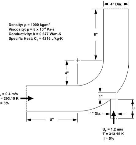
The problem is shown schematically in the figure below. A cold fluid at 293.15 K flows into the pipe through a large inlet and mixes with a warmer fluid at 313.15 K, which enters through a smaller inlet located at the elbow. The mixing elbow configuration is encountered in piping systems in power plants and process industries. It is often important to predict the flow field and temperature field in the area of the mixing region in order to properly design the junction.
Solution:
Start ANSYS Workbench by clicking the Windows Start menu, then selecting the Workbench 14.0 option in the ANSYS 14.0 program group.
Start → All Programs → ANSYS 14.0 → Workbench 14.0
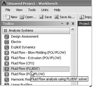
This displays the ANSYS Workbench application window, which has the Toolbox on the left and the Project Schematic to its right. Various supported applications are listed in the Toolbox and the components of the analysis system will be displayed in the Project Schematic.
Create a new FLUENT fluid flow analysis system by double-clicking the Fluid Flow (FLUENT) option under Analysis Systems in the Toolbox.
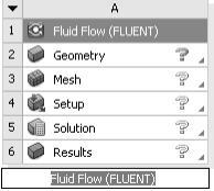
This creates a new FLUENT-based fluid flow analysis system in the Project Schematic.
Name the analysis:
- Double-click the Fluid Flow (FLUENT) label underneath the analysis system (if it is not already highlighted).
- Enter ‘elbow’ for the name of the analysis system.
Save the project:
- Select the Save option under the File menu in ANSYS Workbench (File → Save).
- In your working directory, enter ‘elbow-workbench’ as the project file name and click the Save button to save the project. ANSYS Workbench saves the project with a .wbpj extension and also saves supporting files for the project.
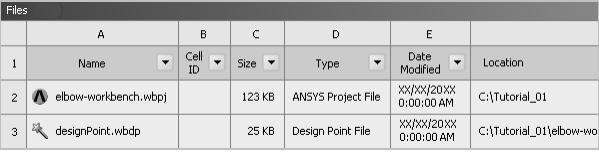
View the list of files generated by ANSYS Workbench.
ANSYS Workbench allows you to easily view the files associated with your project using the Files view. To open the Files view, select the Files option under the View menu at the top of the ANSYS Workbench window (View → Files).
In the Files view, you will be able to see the name and type of file, the ID of the cell that the file is associated with, the size of the file, the location of the file, and other information. For more information about the Files view, see Files View.
For the geometry of your fluid flow analysis, you can create a geometry in ANSYS Design Modeler, or import the appropriate geometry file. In this step, you will create the geometry in ANSYS Design Modeler, then review the list of files generated by ANSYS Workbench.
Design Modeler
Start ANSYS Design Modeler.
In the ANSYS Workbench Project Schematic, double-click the Geometry cell in the elbow fluid flow analysis system. This displays the ANSYS Design Modeler application.
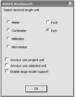
Set the units in ANSYS Design Modeler.
Create the geometry
The geometry for this tutorial consists of a large curved pipe accompanied by a smaller side pipe. To create the larger main pipe, you will use the Sweep operation. Sweeping requires the use of two sketches: one that defines the profile to be swept and the other that defines the path through which the profile is to be swept. In this case, the profile is a half circle because the symmetry of the problem means that you do not have to generate the entire pipe geometry.
Create a new plane by selecting YZPlane from the Tree Outline, then clicking the New Plane icon in the Active Plane/Sketch toolbar near the top of the ANSYS Workbench window. Selecting YZPlane before you create the new plane ensures that the new plane is based on the YZPlane.
In the Details View for the new plane (Plane4), set Transform1 (RMB) to Offset Global X by clicking the word None to the right of Transform1 (RMB) and selecting Offset Global X from the drop-down menu. Set the Value of the offset to -8 in by clicking the 0 to the right of FD1, Value 1 and entering -8. Note that the inch’s measurement appears automatically when you click outside of this box.

To create the plane, click the Generate button which is located in the ANSYS Design Modeler toolbar.
Create a new sketch by selecting Plane4 from the Tree Outline and then clicking the New Sketch icon in the Active Plane/Sketch toolbar, near the top of the ANSYS Workbench window. Selecting the plane first ensures that the new sketch is based on Plane4.
On the Sketching tab of the Tree Outline, open the Settings toolbox, select Grid, and enable the Show in 2D and the Snap options.
Set Major Grid Spacing to 1 inch and Minor-Steps per Major to 2.
Create the profile: Zoom in on the center of the grid so that you can see the grid lines clearly. You can do this by holding down the right mouse button and dragging a box over the desired viewing area.
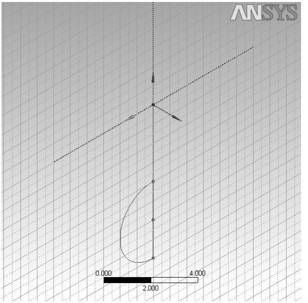
On the Sketching tab, open the Draw toolbox and select Arc by Center (you may need to use the arrows in the toolbox to scroll down to see the correct tool). You will be drawing an arc with a radius of 2 inches, centered on Y=- 6 inches, Z=0 inches (located below the origin of Plane4). The grid settings that you have just set up will help you to position the arc and set its radius correctly.
To create the arc, click the point where you want to create the center of the circle (in this case, Y=- 6 inches, Z=0 inches). Then click the point where you want to start drawing the arc (in this case Y=- 4 inches, Z=0 inches). At this stage, when you drag the unclicked mouse, Design Modeler will create an arc with a fixed radius. With the mouse button unclicked, drag through an arc of 180°. Click on Y=- 8 inches, Z=0 inches to stop the drawing process.
Next, you will close the half-circle with a line that joins the two arc ends. On the Sketching tab, in the Draw toolbox, select Line (you may need to use the arrows in the toolbox to scroll up to see the correct tool). Draw a line from Y=- 4 inches, Z=0 inches to Y=- 8 inches, Z=0 inches. This closed half-circle will be used as the profile during the sweep.