In this guide, we will solve the problem of loss of head in the pipeline and will discuss how to calculate head loss. This sample will help you understand how the flow resistance is going. On real numbers, we will describe the algorithm for how to do this. We use the basic formulas. We will examine a simple example with a pipe, as seen in the image at the beginning of the sample. After you read through our example, you will know how to calculate head loss.
By the end of the sample, you will understand how to deal with your own assignment. The guide is quite simple, so you can easily use it to solve your problem. In general, there is not an easy way to recognize the head loss, but our example presents the most basic one. The method that is presented in the sample is offered by an expert in engineering. Let’s find out what this method is!
Head Loss Calculation
Task: in this guide we will perform m head loss calculations, solve flow rate problems, generate system curves, and find the design point for a system and pump for pipe flow analysis.
Solution:
(Part 3)
Head Loss Computation
The simplest pipe flow problem involves computing the head loss when the pipe diameter and the flow rate are known.
function HLC
% — Define constants for the system and its components
L = 0.1; % Pipe length (m)
D = 4e-3; % Pipe diameter (m)
A = 0.25*pi*D.^2; % Cross sectional area
e = 0.0015e-3; % Roughness for drawn tubing
rho = 1.23; % Density of air (kg/m^3) at 20 degrees C
g = 9.81; % Acceleration of gravity (m^2/s)
mu = 1.79e-5; % Dynamic viscosity (kg/m/s) at 20 degrees C
nu = mu/rho; % Kinematic viscosity (m^2/s)
V = 50; % Air velocity (m/s)
% — Laminar solution
Re = V*D/nu;
flam = 64/Re;
dplam = flam * 0.5*(L/D)*rho*V^2;
% — Turbulent solution f = moody(e/D,Re);
dp = f*(L/D)*0.5*rho*V^2;
% — Print summary of losses
fprintf(’\nMYO Example 8.5: Re = %12.3e\n\n’,Re);
fprintf(’\tLaminar flow: ’);
fprintf(’flam = %8.5f; Dp = %7.0f (Pa)\n’,flam,dplam)
fprintf(’\tTurbulent flow: ’);
fprintf(’f = %8.5f; Dp = %7.0f (Pa)\n’,f,dp);
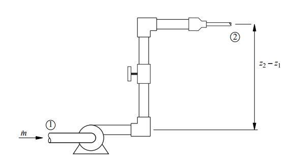
Head loss problems are slightly more complicated when multiple pipe segments and multiple minor loss elements are connected in a series. The calculations are more tedious than difficult, and a computer tool can relieve the tedium. A general procedure can be developed by considering the system. The system consists of six pipe segments with lengths L1,2, L2,3, L3,4, L4,5, L5,6, L6,7 and diameters D1,2, D2,3, D3,4, D4,5, D5,6, D6,7. In general, each pipe segment could be made of a different material, so each segment could potentially have a different wall roughness. The system in Figure 4 also has four minor loss elements: elbows at stations 3 and 5, a valve at station 4, and a reducer at station 6. Applying Equation (8) to the system in Figure 4 gives the total head loss from station 2 to station 7:
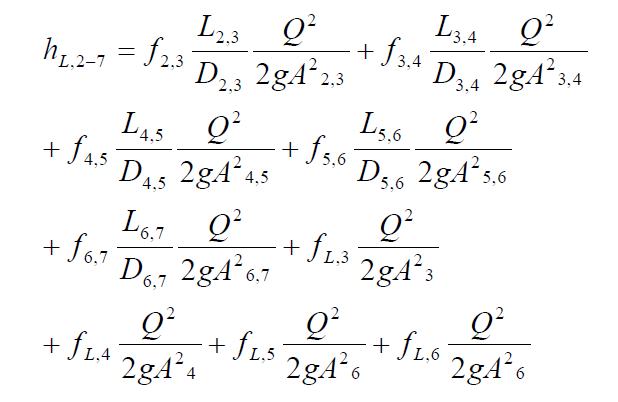
Notice that the flow rate, Q, is common to all terms. Also notice that the viscous terms involve the product of Q2 with f, which is also a function of Q, because Q determines the Reynolds number.