Are you tired from looking for good root locus method examples? Congratulations! You don’t have to do this anymore. Below, you’ll find an example that will surely help you with your own task. It was completed by an expert from AssignmentShark. All of our experts have vast experience in doing tasks of this kind, and have graduated from their educational affiliations.
If you need to get help with any of your tasks, feel free to fill the order form on our website. We’ll be glad to cope even with the most challenging and urgent tasks. AssignmentShark is a service which helps with assignments in technical disciplines, such as programming, engineering, physics, and others. Do you want to have root locus method examples completed just for you as soon as possible? Do not hesitate to make the order. Our service is available 24/7!
Task:
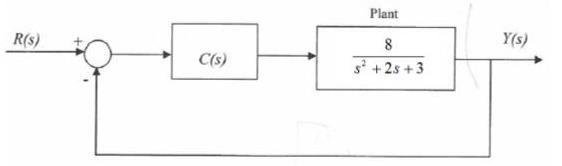
Design the P, PD, PI, and PID controllers and analyze their characteristics for following the block diagram. The designed controller must provide stability, settling time of less than 0.6 seconds, and peak overshoot less than 8%.
Solution:
Root locus design is a common control system design technique in which you edit the compensator gain, poles, and zeros in the root locus diagram.
As the open-loop gain (k) of a control system varies over a continuous range of values, the root locus diagram shows the trajectories of the closed-loop poles of the feedback system. For example, look at the following tracking system:
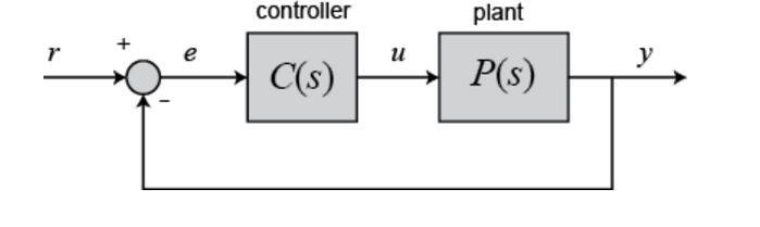
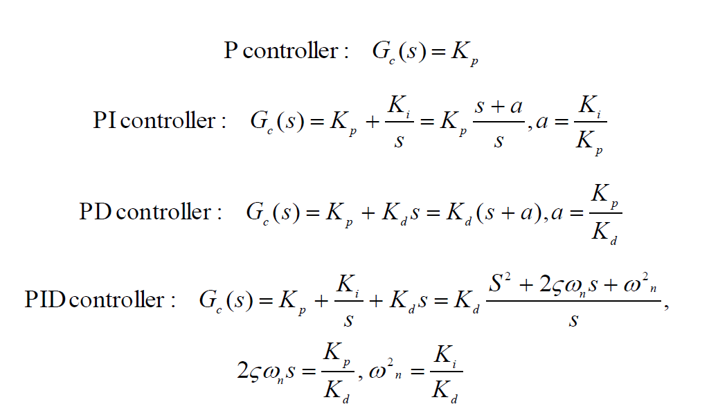
The variable (e) represents the tracking error, the difference between the desired input value (r) and the actual output (y). This error signal (e) will be sent to the PID controller, and the controller computes both the derivative and the integral of this error signal. The control signal (u) to the plant is equal to the proportional gain (Kp) times the magnitude of the error plus the integral gain (Ki) times the integral of the error plus the derivative gain (Kd) times the derivative of the error.
A proportional controller (Kp) will have the effect of reducing the rise time and will reduce but never eliminate the steady-state error.
An integral control (Ki) will have the effect of eliminating the steady-state error for a constant or step input, but it may make the transient response slower.
A derivative control (Kd) will have the effect of increasing the stability of the system, reducing the overshoot, and improving the transient response.
Results for the mentioned controllers are listed below.
P controller
Of all the controllers to control a system, the proportional controller is the simplest of them all. A proportional control system amplifies the error signal to generate the control signal. In other words, a proportional controller is just an amplifier.
By using Matlab, we get the next plots:
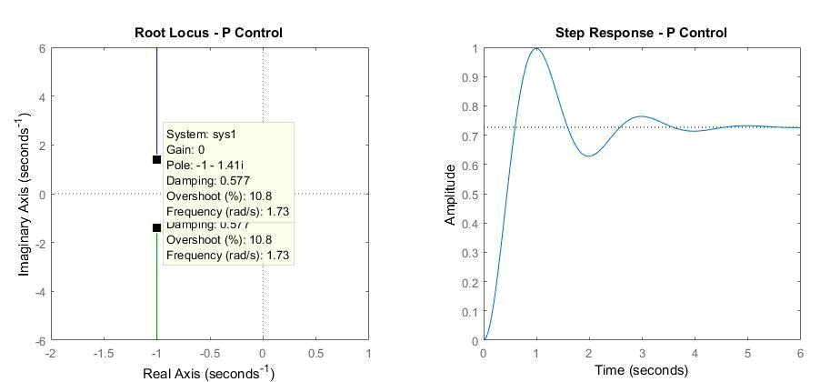
Figure 2: P controller
From the plots above, we can conclude that the system is stable since the two mating lines that represent k values are not moving in the unstable region (right part of x axis), but minimum overshoot is 10.8% (required < 10%) and settling time is a constant 4s (required <0.5s).
PI controller
Using PI adds a zero to the open-loop system. We’ll place this zero at 8. The zero must lie between the open-loop poles of the system, in this case so that the closed-loop system will be stable.
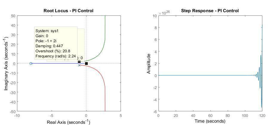
Figure 3: PI controller
From the plots above, we can conclude that the system is unstable since the two mating lines are moving in the unstable region (right part of x axis), also minimum overshoot is 20.8% (required < 8%) and settling time will increase since going to the unstable area.
PD controller
The compensated system open-loop transfer function will have one additional zero. The effect of this zero is to introduce a positive phase shift. Let’s make the value of zero to be a distance away by selecting 40.

Figure 4: PD controller
From the plots above, we can conclude that the system is stable since it is located in the stable region, minimum overshoot is 0.901% (required < 8%) and settling time is bigger than 0.6s (8rad/s).
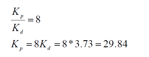
Kp can be found as ( Kd = 2.57 (gain value from plot) ):
PID controller
In order to pull the root locus further to the left, to make it faster, we need to place a second open-loop zero, resulting in a PID controller. After some experimentation, we place the two PID zeros at s1 20 and s2 20 .
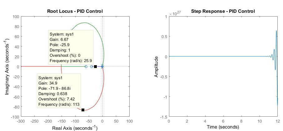
Figure 5: PID controller
From the plots above, we can conclude that the system is stable since it is located in the stable region, minimum overshoot is 7.42% (required < 8%) and settling time is bigger than 0.6s (8rad/s).
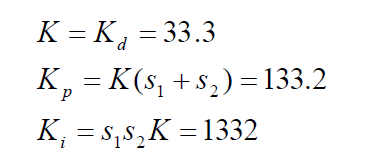
Now let’s calculate the gain values K, Kd, Ki, Kp:
As we can see from the graph above, it was possible to calculate the precise location of the roots, and to choose a value of K that gave us a good response from proportional, integral, derivative, and PID controllers. Then by variating the proportional, integral, and derivative gains, we looked at how response was changing. As we expected, PID response has an overshoot of less than 8% and a settling time less than 0.6 seconds and fits all mentioned design specifications.
Also, we can see advantages of root locus technique, such as:
- The root locus technique in a control system is easy to implement as compared to other methods.
- Root locus provides the better way to indicate the parameters.
- With the help of root locus we can easily predict the performance of the whole system.